Creative Commons license

Copyright notice: I hereby release all of the writing  content that is tagged by R, under the cc-by-sa copyrights (date: Jan 26 2012), as long as the copied content comes with proper attribution which also  includes a link to the source of the article .

India Census 2001 – Part 1

I was trying – for the last few weeks – to get the 2001 Indian census data. Alas the census website is under construction. But fortunately the Internet rewind button works! Thankfully the literacy data was online there. The raw data is available here.

I cleaned up the data so that it is easy to work with R. I removed the commas in the numbers. Also, under the urban status column I removed the dots and capitalized the status codes. One of the urban status became ‘NA’ and since R treats ‘NA’ as a missing data I changed it to NA1.

The cleaned up data is available here. Please download and rename it as india-census-2001.csv

Here goes the R code to explore the data:

#---------------------------------------------------------------------------
# set the working directory
# replace dir with your own path where "india-census-2001.csv" is stored
setwd("dir")

# load the plotting package
library(lattice)
india <- read.csv(file = "india-census-2001.csv", header = T)

# find out the places with zero population!
india_pop_zero <- subset(india, TotPop == 0)[,c(2,3,4,5)]
#---------------------------------------------------------------------------

Lets us print out those places with zero population.

#---------------------------------------------------------------------------
print(india_pop_zero)
           City UrbanStatus   State District
200       Anjar           M Gujarat  Kachchh
636     Bhachau           M Gujarat  Kachchh
735        Bhuj           M Gujarat  Kachchh
1495 Gandhidham           M Gujarat  Kachchh
2173     Kandla          CT Gujarat  Kachchh
2937     Mandvi           M Gujarat  Kachchh
3128      Morvi           M Gujarat   Rajkot
3178     Mundra          CT Gujarat  Kachchh
4043      Rapar           M Gujarat  Kachchh
5119   Wankaner           M Gujarat   Rajkot
#---------------------------------------------------------------------------

Find out the population in all Kachchh districts.

#---------------------------------------------------------------------------
subset(india, District == "Kachchh")[,c(2,3,4,5,6)]
           City UrbanStatus   State District TotPop
200       Anjar           M Gujarat  Kachchh      0
636     Bhachau           M Gujarat  Kachchh      0
735        Bhuj           M Gujarat  Kachchh      0
1495 Gandhidham           M Gujarat  Kachchh      0
2173     Kandla          CT Gujarat  Kachchh      0
2937     Mandvi           M Gujarat  Kachchh      0
3178     Mundra          CT Gujarat  Kachchh      0
4043      Rapar           M Gujarat  Kachchh      0
#---------------------------------------------------------------------------

Find out the population in all Rajkot districts.

#---------------------------------------------------------------------------
> subset(india, District == "Rajkot")[,c(2,3,4,5,6)]
                City UrbanStatus   State District TotPop
695       Bhayavadar           M Gujarat   Rajkot  18246
1298         Dhoraji           M Gujarat   Rajkot  80807
1613          Gondal           M Gujarat   Rajkot  95991
1956          Jasdan           M Gujarat   Rajkot  39041
1984 Jetpur Navagadh           M Gujarat   Rajkot 104311
3128           Morvi           M Gujarat   Rajkot      0
3521        Paddhari          CT Gujarat   Rajkot   9225
3967          Rajkot       MCorp Gujarat   Rajkot 966642
4919          Upleta           M Gujarat   Rajkot  55341
5119        Wankaner           M Gujarat   Rajkot      0
#---------------------------------------------------------------------------

Looks as if the data in the Kachchh region was not collected. Wonder why those two Rajkot districts also suffered the unfortunate fate. Maybe they are close to Kachchh region. Anyway let us look at the data which has non-zero population.

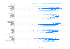
Let us plot the literacy rate of the city/town (x-axis) against the State (y-axis)

#---------------------------------------------------------------------------
india <- subset(india, TotPop > 0)
# Plot the literacy data
dotplot(State ~ 100*Literates/TotPop, xlab = "Literacy", data = india)
#---------------------------------------------------------------------------

Here goes the plot

Looking at the plot, no surprise that Kerala has very high literacy rate in all the towns and the spread is also low. Tamil Nadu has a bigger spread in the literacy rates. The Northeastern states are doing very well in the educational aspect if we evaluate them by their literacy rates.

Let us check which city/town has the highest and the lowest literacy in India

#---------------------------------------------------------------------------
subset(india, TotLiteracy == max(TotLiteracy))[,c("City", "State", "District", "TotLiteracy")]
        City           State District TotLiteracy
1663 Gulmarg Jammu & Kashmir Baramula    96.23494
#---------------------------------------------------------------------------
subset(india, TotLiteracy == min(TotLiteracy))[,c("City", "State", "District", "TotLiteracy")]
        City       State District TotLiteracy
4666 Tarapur Maharashtra    Thane   0.7843697
#---------------------------------------------------------------------------

Well, this is a surprise. The city with the highest literacy is in Jammu & Kashmir (Gulmarg) and the lowest is in Maharashtra (Tarapur). What is shocking is that the literacy rate in Tarapur is less than 1%. I hope that there was mistake in data collection, otherwise it is a damning indictment of a huge administrative failure in that district. This is unacceptable.

In the next few posts, I will concentrate on Tamil Nadu and Coimbatore. It should be pretty easy to modify the code in the coming posts to look at the states and districts of your interest.

NREGA and Indian maps in R

A few days ago I was reading an article by Jean Drèze and his colleagues on how the first two years of National Rural Employment Guarantee Act (NREGA) has progressed (There was another article by Drèze on NREGA in 2007). The NREGA is empowering the rural people in a radical way:

[ …] NREGA programmes visualise a decisive break with the past. Ever since independence, rural development has largely been the monopoly of local contractors, who have emerged as major agents of exploitation of the rural poor, especially women. Almost every aspect of these programmes, including the schedule of rates that is used to measure and value work done, has been tailor-made for local contractors. These people invariably tend to be local power brokers. They implement programmes in a top-down manner, run roughshod over basic human rights, pay workers a pittance and use labour-displacing machinery.

NREGA is poised to change all that. It places a ban on contractors and their machines. It mandates payment of statutory minimum wages and provides various legal entitlements to workers. It visualises the involvement of local people in every decision — whether it be the selection of works and work-sites, the implementation of projects or their social audit.

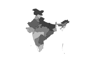
After going through the articles I thought about reproducing the color (gray) coded maps. Of course the best tool to do this would be R. It took a few days to figure out how to do this. The rest of the post (hopefully clearly) will be on how to produce an Indian map gray coded with literacy rate of the state.

• I assume you have R installed. If not please go to http://cran.r-project.org/ and install R.
• Next you have to install a CRAN package maptools.
  • Instructions on installing packages is here.
• If you want a quick introduction to R, I would recommend this terrific tutorial which uses baseball statistics for illustration.
  • If you want a more detailed coverage, Ross Ihaka’s introductory course is the best.

Now on to the exciting part of producing Indian maps:

• First we need an Indian map. Fortunately there is a free Indian map although it is little old. You can download the Indian map from here.
  • Extract the zip file in an directory and let us call this directory “dir”
• I got the literacy data [PDF] from the Indian Budget website and put it as a csv file here. Please download it and rename it as literacy.csv and place it in the same directory (“dir”) as the maps.
  • Note: I removed a few states (Jharkhand, Chhattisgarh, Uttaranchal) from the original data since the Indian map we have is little dated and does not contain these states. Maybe later on we can figure out how to draw the boundaries for those states.

The code is straightforward. I adapted the code from http://r-spatial.sourceforge.net/gallery/ more specifically fig14.R there.

#---------------------------------------------------------------------------
# packages for manipulating and mapping spatial data
library(maptools)
# set the working directory
# replace dir with your own path
setwd("dir")
# read the shapefile with the digital boundaries
india <- readShapePoly("india_st")
summary(india)
attributes(india)
# read the literacy file
literacy <- read.csv("literacy.csv")
summary(literacy)

rrt <- literacy$X2001
brks <- quantile(rrt, seq(0,1,1/7), na.rm=T)
cols <- grey(2:(length(brks))/length(brks))
dens <- (2:length(brks))*3

plot(india,col=cols[findInterval(rrt, brks, all.inside=TRUE)])
#---------------------------------------------------------------------------

Here is the output if everything goes fine. Darker shades means dire literacy levels.

Coimbatore Weather and Questioning Amma!

A week ago, Amma was telling the weather was getting hot in Coimbatore. I was telling her it is going to get worse in the next two months. She shot back saying that March is the hottest month while April and May are less hotter in Coimbatore. Growing up in India you are thought that your mother knows the best and she is right (almost) always. Well I could not resist the thought of putting the thesis to test and the internet comes to my help. So here goes the perl and R code to  get the temperature data and explore it. The metric of choice would (arbitrarily) the average temperature. In R plots in this post the average is plotted by a big black dot. The month with the highest average temperature will be adjudged the hottest month. There are a lot of metrics to use but this is the simplest and the most intuitive.

(1)  perl code to scrap temperature data from web. The wunderground website has data in csv format. I did not do checks like limiting days in June to 30. We will fix that in clean up script which will build a single csv file with data from years 2005 to 2008. You need the CPAN package LWP.You should be able to google and figure out how to install LWP package.

Save this file as [dir]/src/get_temperature_files.pl
To run
% cd [dir]/src
% perl get_temperature_files.pl
You will have the data in the directory [dir]/data
The data is for four years from 2005 to 2008.

#------------------------------------------------------------------
use warnings;
use strict;
#------------------------------------------------------------------
use LWP::UserAgent;
#------------------------------------------------------------------
@ARGV == 0 or die "Sorry. The correct usage is:\
       perl get_temperature_files.pl\n";
#------------------------------------------------------------------

my $datadir = "../data/";
mkdir($datadir, 0755) unless -d $datadir;
# VOCB - Coimbatore
my $base_url =  "http://www.wunderground.com/history/airport/VOCB/";
my $suffix = "/DailyHistory.html?format=1";

for (my $year = 2005; $year < 2009; ++$year) {
  for (my $month = 1; $month <= 12; ++$month) {
    for (my $day = 1; $day <= 31; ++$day) {
      my $webfile = $year."/".$month."/".$day;
      print "Getting: $webfile\n";

      my $url = $base_url.$webfile.$suffix;
      my $webPage = getWebPage($url);

      my $outfile = $year."_".$month."_".$day.".csv";
      $outfile = $datadir.$outfile;
      open(OUTFILE, ">$outfile");
      print OUTFILE "$webPage";
      close(OUTFILE);

# let us be patient and decent
      sleep(1);
    }
  }
}

#------------------------------------------------------------------
# subroutines
#------------------------------------------------------------------
sub getWebPage {
  my ($url) = @_;
  my $browser = LWP::UserAgent->new();
  my $response = $browser->get($url);

# error checks
  die "Weird content type at $url -- ", $response->content_type()
    unless $response->is_success();

  my $webPage = $response->content();
  return($webPage);
}
#------------------------------------------------------------------

(2) Clean up the data and construct the data as a single file.
Save this file as [dir]/src/build_csv.pl
To run
% cd [dir]/src
% perl build_csv.pl ../data/ > cbe.csv

#------------------------------------------------------------------
use warnings;
use strict;
#------------------------------------------------------------------
@ARGV == 1 or die "Sorry. The correct usage is:\
       perl build_csv.pl dir_containing_csv_files\
       Example:\
       perl build_csv.pl ../data/\n";
#------------------------------------------------------------------
my $datadir = $ARGV[0];
# make sure exactly one / is present after $datadir
$datadir =~ s/[\/]+$//;
$datadir .= "/";

# days in a month
my @days_in_month  = (31,28,31,30,31,30,31,31,30,31,30,31);
my @month_names = ("Jan", "Feb", "Mar", "Apr", "May", "Jun",
    "Jul", "Aug", "Sep", "Oct", "Nov", "Dec");

opendir(DIR, $datadir);
my @files = grep { /\.csv$/ } readdir(DIR);
closedir(DIR);

my $header_flag = 0;
foreach (@files) {
  my $file = $_;

# get the time information
# which we need to add to the csv file
  my ($time, $suffix) = split(/\./, $file);
  my ($year, $month, $day) = split(/\_/, $time);

# handle leap year
  if (0 == $year % 4) {
    $days_in_month[1] = 29;
  } else {
    $days_in_month[1] = 28;
  }

  if ($day <= $days_in_month[$month-1]) {
# read the raw csv file and clean it up
    my $csvfile = $datadir.$file;
    open(TIMEFILE, "<$csvfile");

    while () {
# remove everything between and including < >
      s/\<.*\>//;
# skip blank lines
      next if /^(\s)*$/;

# skip the header after the printing it
# for the first time
      if(!$header_flag) {
        print "year, month, day, $_";
        $header_flag = 1;
        next;
      } else {
        next if /^[a-z]+.*$/i;
      }

      chomp;
      print "$year, $month_names[$month-1], $day, $_\n";
    }

    close(TIMEFILE);
  }
}
#------------------------------------------------------------------

(3) Explore the data using R

library(lattice)
# read the raw data
filename <- "cbe.csv";
x <- read.csv(file = filename, header = TRUE, as.is = TRUE);

# factor hack to get the plots in xyplot() in correct order
x$month = factor(x$month, levels=x$month)
x$year = factor(x$year, levels=x$year)
x$TimeIST = factor(x$TimeIST, levels=x$TimeIST)
x$TemperatureC = (x$TemperatureF - 32)*(5.0/9.0);

Now for answering the question at the top of the post.

hyear <- bwplot(TemperatureC ~ month | year, data=x, ylab = "Temperature (C)");
plot(hyear);

Looks as if Amma thesis is probably rejected! Four years worth data shows that highest average temperature is in April. Let us see a split by years and see if there is a year in which March’s average temperature was the highest. Looks like we need to do little clean up of the data. There is a zero in October. Definitely not possible in Coimbatore!

hmonth <- bwplot(TemperatureC ~ month, data=x, ylab = "Temperature (C)");
plot(hmonth);

Well it looks like at least in 2005 and 2007 March’s average temperature is the highest. Although April matches March in both those years. I am trying to find something to salvage for my Amma!

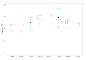
Here is an another plot which splits by the hour of the day.

hhour <- bwplot(TemperatureC ~ TimeIST, data=x, ylab = "Temperature (C)");
plot(hhour);

The one surprising thing one was the fact that the lowest temperatures occur between 2:30 AM and 5:30 AM not around midnight. The highest temperatures are around 2:30 PM not noon. Well the zero is definitely an error since it shows up at 11:30 AM.

Update 1 (March 16 2009):

You can download [~700 KB, rename it as cbe.csv] the big csv file which contains the data for the weather in Coimbatore for years 2005 — 2008. Now you can skip to the Step (3) and use R to analyze the data.